Importing necessary modules
import numpy as np
import matplotlib.pyplot as pltAs it is known, machine learning techniques try to model a certain function \(f(x)\) (or \(y\)) based on certain training data, that consists on known \(f(x)\) (output) values for certain \(x\) (input) points.
In order to tackle this problem, one can make assumptions on the underlying function behind \(f(x)\), for example a linear function:
\[ f(x) = a \cdot x + b \]
or a quadratic function
\[ f(x) = a\cdot x^2 + b\cdot x + c \]
or as complex as needed. The approximation in those cases is known as parametric regression because the parameters (e.g. \(a\), \(b\), \(c\), … ) will be estimated so that the difference between the function to approximate (\(f(x)\)) and our model minimizes the root mean square error (RMSE).
But, what happens if we do not know the underlying function? In this case, one can rely on Gaussian Processes (GPs), which offer a way to model \(f(x)\) in a probabilistic, non-parametric manner, avoiding assumptions about its analytic form (see for instance Section 15.9 of Press (2007)).
In order to understand how GP work, it is important to think of \(f(x)\), not as a continuous, closed-form, analytical expression such as, for example:
\[ f(x) = -x^3+5\cdot x^2 - \frac{x}{2} -1 \]
but rather, as a set of probabilistic relationships between the function values. These relationships are provided by the kernel, which quantifies how the values of \(f(x)\) for the different inputs (\(x\)) are related. The kernel (or set of covariances) is computed based on the training data set. As an example, for the function given above, a possible training dataset could be (see Figure 1):
import numpy as np
import matplotlib.pyplot as pltdef f(x: np.array) -> np.array:
return -1 * np.power(x, 3) + np.power(x, 2) * 5 - x * 0.5 - 1
x = np.array([0. ,1.67 , 3.33 , 5.0 ])
y = f(x)formatter= {'float_kind': lambda x: "%7.2f" % x}
print(np.array2string(x, precision=2, separator=',', formatter=formatter))
print(np.array2string(y, precision=2, separator=',', formatter=formatter))[ 0.00, 1.67, 3.33, 5.00]
[ -1.00, 7.45, 15.85, -3.50]Once the kernel has been computed using the training data set, one can obtain the value of \(f(x)\) at an arbitrary point within the domain specified by the training data. An important feature that the GP offer is the provision of not only the value of the \(f(x)\) but also its formal uncertainty.
fig = plt.figure(figsize=(9, 5))

plt.title("Example of f(x)")
ax = fig.gca()

x_continuous = np.linspace(0, 5, 100)
ax.plot(x_continuous, f(x_continuous), label="continuous")
ax.set_xlabel('x')
ax.set_ylabel('f(x)')


x_discrete = x
ax.plot(x_discrete, f(x_discrete), "or", label="training dataset")

ax.legend()

plt.show()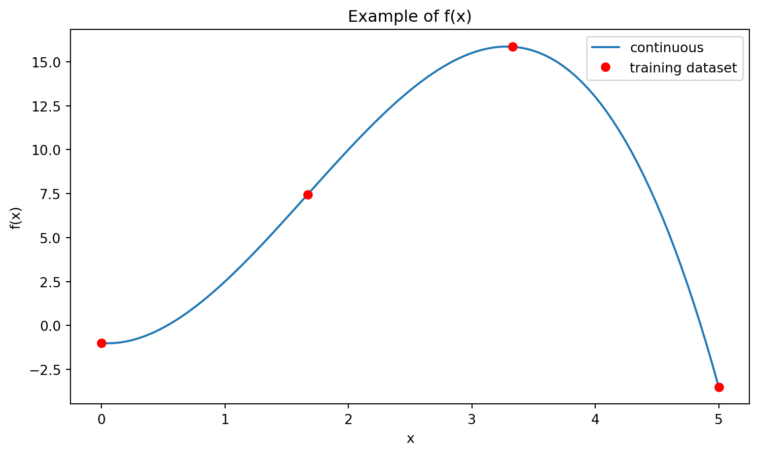
This post tries to reproduce the pictorial introduction of Gaussian Processes shown in Figure 1.1 of Williams and Rasmussen (2006) and is organized as follows: the first section will illustrate how a kernel is computed, using the GP equations, and the subsequent section will use an external library to train a GP (not only computing the kernel but also optimizing any hyperparameters set for the model).
Before showing how the kernel is computed, let’s first get an understanding on the meaning of “drawing a number of sample functions at random from the prior distribution”.
Let’s assume that the output function is actually an array (not a continuous function) of \(N\) points, i.e.
\[ f(x) = \{y_1, y_2, y_3, ...y_N\} \quad for \quad x = \{x_1, x_2, x_3, ... x_N\} \]
Then we assume that the array \(f(x)\) can be modelled as a set of random variables with a Gaussian distribution (i.e. multivariate Gaussian distribution), where the individual data points are not independent (i.e. covariance is not 0). If the points would be independent, this would be equivalent of having \(N\) univariate Gaussian random variables (one per each point), as shown in Figure 2. In this case, each function is in fact \(N\) realizations (one per each point) of a Gaussian distribution, and each point is independent to the previous.
# Define input points (e.g., 100 evenly spaced points in 1D)
X = np.linspace(-5, 5, 100)[:, None]

# Zero mean function for all points (common GP assumption)
mean = np.zeros(X.shape[0])K = np.diag([2.0] * len(mean))
# Draw 5 random function samples from the GP prior (multivariate normal)
samples = np.random.multivariate_normal(mean, K, 5)
plt.figure(figsize=(10, 6))
plt.plot(X, samples.T, lw=1.5)
plt.title('Sample Functions Drawn from GP Prior (Zero Mean, Zero covariance kernel)')
plt.xlabel('x')
plt.ylabel('f(x)')
plt.grid(True)
plt.show()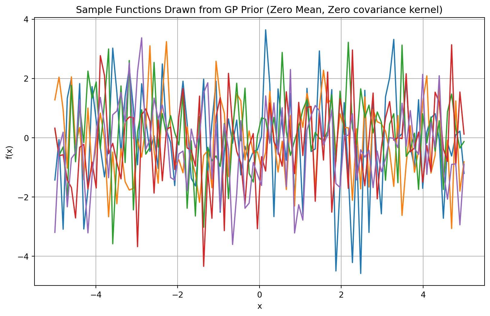
In order to not assume independency betweeen the points (and thus control the smoothness of the function), a kernel (\(K\)) needs to be specified. \(K\) is in fact a matrix containing the covariance of the different data points. For independent data points, the Kernel (\(K\)) would be diagonal (zero covariance). Intuitively, you can interpret the covariance as the similarity between two points of the data set: a smooth function implies that neighbouring points are very similar. In order to compute this covariance (or similarity, \(K({\bf x_1}, {\bf x_2})\)) it is common to use Radial Basis Functions over two arrays (\({\bf x_1}\) and \({\bf x_2}\)):
\[ K({\bf x_1}, {\bf x_2})= \exp \left( -\frac{\| {\bf x_1} - {\bf x_2}\|^2}{2 \sigma^2}\right) \]
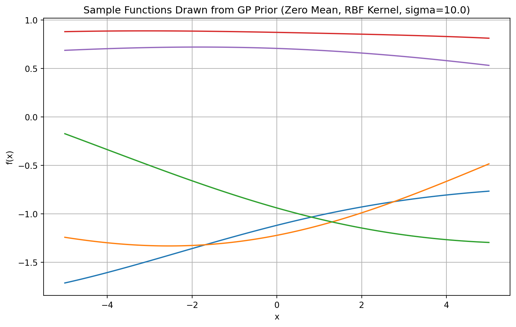
The Kernel function is defined in the rbf_kernel function below. Note that \(\sigma\) controls the smoothnes of the function, the larger the \(\sigma\), the smoother the functions will be, see Figure 3.
def rbf_kernel(x1, x2, sigma=1.0):
    sqdist = np.sum(np.power(x1, 2), 1).reshape(-1, 1) + np.sum(np.power(x2, 2), 1) - 2 * np.dot(x1, np.transpose(x2))
return np.exp(-0.5 / sigma**2 * sqdist)sigma_small = 1.0
K_small = rbf_kernel(X, X, sigma=sigma_small)
sigma_large = 10.0
K_large = rbf_kernel(X, X, sigma=sigma_large)
# Draw 5 random function samples from the GP prior (multivariate normal)
samples_small = np.random.multivariate_normal(mean, K_small, 5)
samples_large = np.random.multivariate_normal(mean, K_large, 5)
plt.figure(figsize=(10, 6))
plt.plot(X, samples_small.T, lw=1.5)
plt.title(f'Sample Functions Drawn from GP Prior (Zero Mean, RBF Kernel, sigma={sigma_small})')
plt.xlabel('x')
plt.ylabel('f(x)')
plt.grid(True)
plt.show()
# Draw 5 random function samples from the GP prior (multivariate normal)
samples = np.random.multivariate_normal(mean, K, 5)
plt.figure(figsize=(10, 6))
plt.plot(X, samples_large.T, lw=1.5)
plt.title(f'Sample Functions Drawn from GP Prior (Zero Mean, RBF Kernel, sigma={sigma_large})')
plt.xlabel('x')
plt.ylabel('f(x)')
plt.grid(True)
plt.show()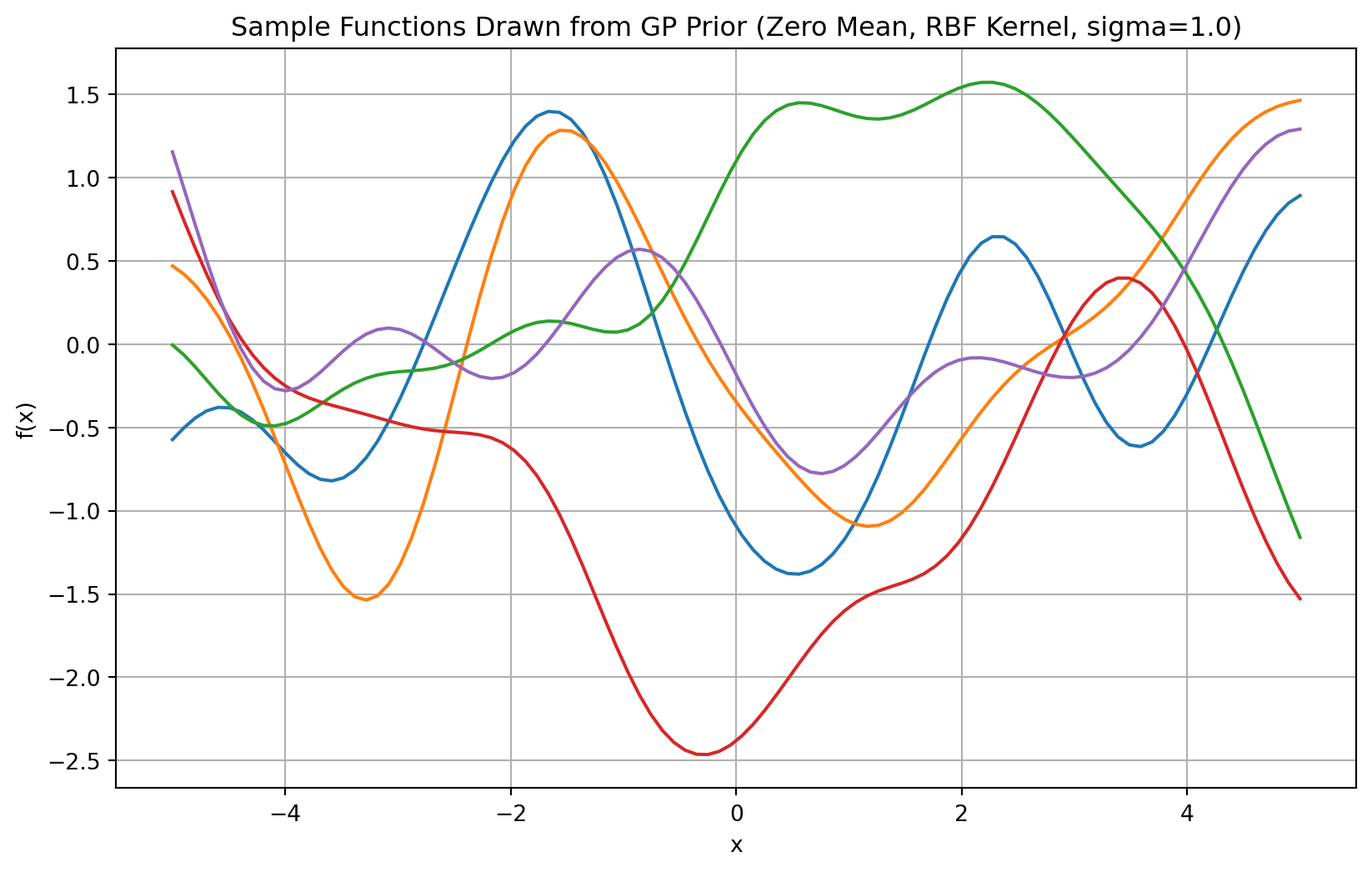
This sections covers the fundamentals of establishing the predictive/posterior mean and variance using a fixed \(\sigma\) (which is in fact a hyperparameter that will be optimized in a training step shown in the following session). Both the predictive/posterior mean and variance can be obtained using the closed-form analytical expression.
Let’s use an observation dataset as follows
X_train = [[-2], [0], [1], [2]]  # List of features
Y_train = [0.5, 1.2, 0.9, 3.3]
Why 2D dimension in X_train? Because X can be considered as an array of features and the distance function (the kernel) computes the distance between arrays of features.
Once the training dataset is defined, the predictive/posterior mean (\(\mu_*\)) as well as the associated predictive/posterior variance (\(\sigma_*^2\)) for a input to be predicted (\(x_*\)) can be computed using the following closed forms
\[ \begin{eqnarray} \mu_* & = & m(x_*) + k_*^T \cdot \hat K \cdot (y-m(X)) \\ \sigma_* & = & k(x_*, x_*)-k_*^T \cdot \hat K \cdot k_* \\ \end{eqnarray} \]
where
\[ \hat K = [K + \sigma_n^2I]^{-1} \]
Note that, to compute the Kernel (\(K\)), two hyperparameters are required:
# Hyperparameters
sigma = 1.0
sigma_n = 1e-4
In this toy example these hyperparameters will be kept fixed, but in a machine learning context, they can be refined using an optimization algorithm such as gradient descent that will lead a set of hyperparameters that minimize the square root mean error.
The different elements in the previous equation are defined and computed as follows
# Compute kernel matrix for training points ($\hat K$)
K_hat = rbf_kernel(X_train, X_train, sigma)
K_hat += sigma_n * np.eye(len(X_train))
K_hat = np.linalg.inv(K_hat)# Prepare Prediction Grid (Test Points)
X_test = np.linspace(-3, 3, 100).reshape(-1, 1) # Predict at 100 evenly spaced pointsK_s) is the vector of covariances between the new test points (\(x_*\)) and the observed input (\(x\)), and is computed as follows:K_s = rbf_kernel(X_train, X_test, sigma)K_ss) the covariance of the test input (\(x_*\)) with itselfK_ss = rbf_kernel(X_test, X_test, sigma)Therefore, the predictive/posterior mean at the test points (\(\mu_*\)) can be computed as:
mu_s = K_s.T @ K_hat @ Y_trainAnd the predictive/posterior covariance at the test points (\(\sigma_*^2\)), which will give an indication of the confidence of the prediction, will be computed as:
cov_s = K_ss - K_s.T @ K_hat @ K_s  # Shape: (100,100)
std_s = np.sqrt(np.diag(cov_s))     # Predictive standard deviation (sigma)
The result of the prediction (for the fixed set of hyperparameters) can be then plotted (see Figure 4), showing that the predicted mean crosses exactly the training points.
import matplotlib.pyplot as plt

plt.figure(figsize=(9, 5))
plt.plot(np.array(X_train).flatten(), Y_train, "ko", label="Train data")
plt.plot(np.array(X_test).flatten(), mu_s, "b", lw=2, label="Posterior mean")
plt.fill_between(
    X_test.flatten(),
    mu_s - 2*std_s, mu_s + 2*std_s,
    color="blue", alpha=0.2, label="Uncertainty (2$\sigma$)"
)
plt.xlabel("x")
plt.ylabel("f(x)")
plt.title("Gaussian Process Regression (Manual Training)")
plt.legend()
plt.grid(True)
plt.show()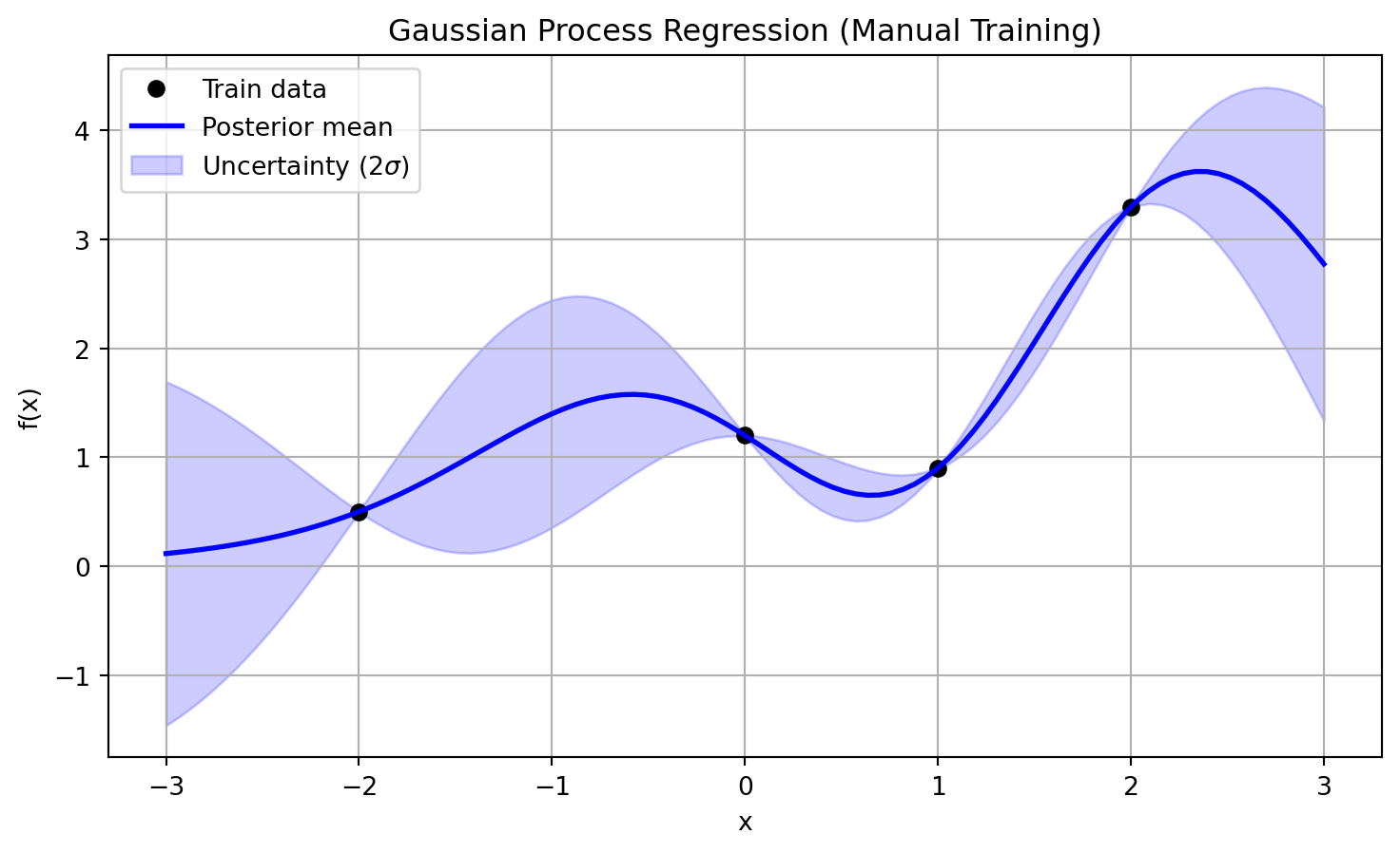
This section will cover the usage of sklearn package in order to train the Gaussian Process and obtain a refined set of hyperparameters that minimises the root mean squared error (RMSE).
As the kernel function, we will use sklearn’s RBF class, which actually implements the rbf_kernel function shown above. Note that in the GaussianProcessRegressor class, it is possible to specify the alpha parameter, which can be interpreted as the variance of a Gaussian noise (\(\sigma_n\)).
from sklearn.gaussian_process import GaussianProcessRegressor
from sklearn.gaussian_process.kernels import RBF

kernel = 1 * RBF(length_scale=1.0, length_scale_bounds=(0.01, 100))
gaussian_process = GaussianProcessRegressor(kernel=kernel, alpha=sigma_n**2, n_restarts_optimizer=9)
gaussian_process.fit(X_train, Y_train)
gaussian_process.kernel_
1.79**2 * RBF(length_scale=0.664)mu_s_hyper, std_s_hyper = gaussian_process.predict(X_test, return_std=True)In Figure 5, the result of this training is being shown (in addition, the result using manual training is also provided for reference). Note that in the positions of the training data set, there is also a certain uncertainty level that matches the \(\sigma_n\) value specified before. If this value is increased, the uncertainty level of the prediction will increase accordingly.
plt.figure(figsize=(9, 5))
plt.plot(np.array(X_train).flatten(), Y_train, "ko", label="Train data")
plt.plot(np.array(X_test).flatten(), mu_s, "b", lw=2, label="Posterior mean")
plt.fill_between(
    X_test.flatten(),
    mu_s - 2*std_s, mu_s + 2*std_s,
    color="blue", alpha=0.2, label="Uncertainty (2$\sigma$)"
)
plt.plot(np.array(X_test).flatten(), mu_s_hyper, "r", lw=2, label="Posterior mean (with training)")
plt.fill_between(
    X_test.flatten(),
    mu_s_hyper - 2*std_s_hyper, mu_s_hyper + 2*std_s_hyper,
    color="red", alpha=0.2, label="Uncertainty (2$\sigma$, with training)"
)
plt.xlabel("x")
plt.ylabel("f(x)")
plt.title("Gaussian Process Regression (with Training)")
plt.legend()
plt.grid(True)
plt.show()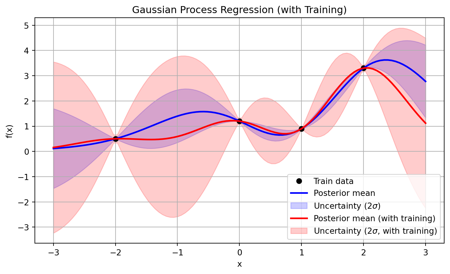
This post attempted to provide with a very basic introduction on the fundamental concepts of the GP so that the reader may be able to build upon more complex scenarios and datasets, and also exploring potential limitations of the technique. One basic drawback of the GP processes is in fact that large training data sets may become impractical due to the fact that computing the Kernel function involves inverting a potentially large matrix (that grows with the size of the input data).
IA tools (Perplexity) has been used to polish grammar and correct typos in the text. In addition, several code snippets have been created with AI as a starting point for implementation. Review and code refinements have been made by the author.